Note: this article is also available in Italian as a PDF file.

Introduction

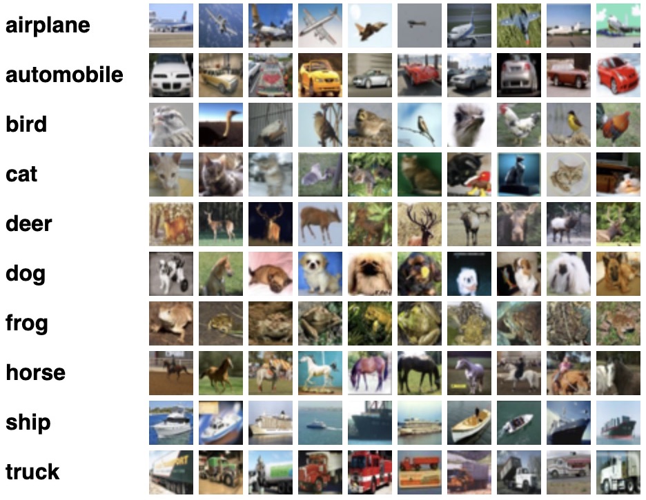
In an Image Classification task, the goal is to attribute to an image one of the labels among those available. Unlike many other classic computer vision tasks, this is the only information we need: we don’t have to tell where the object is in the image with a bounding box, nor define membership classes pixel by pixel. One image, one class among a set of predefined classes, with no overlap. The dataset used in this project is CIFAR-10, containing 60000 color images of size 32x32 pixels¹. One of the peculiarities of this dataset is that, visually, the classes are completely mutually exclusive; the same image will never contain both a car and a truck, two of the categories of images featured in the dataset. It was created as a subset of the 80 Million Tiny Images dataset², and it is widely used for benchmarking vision algorithms. The featured classes are airplanes, cars, birds, cats, deer, dogs, frogs, horses, ships and trucks; the dataset is also artificially balanced, with 6000 images per class, so we will not have any problems related to class imbalance during classification. For all the reasons just listed, it is a dataset commonly used as a benchmark for classification algorithms; its regular structure allows excellent repeatability of the experiments and makes it easy to compare similar metrics across multiple architectures. In our case, to address the classification task, we are going to use two different convolutional network architectures. We will see a first approach that makes use of transfer learning, employing the ResNet-18 convolutional network as a pre-trained feature extractor, and a second, custom convolutional network architecture made ad hoc for the problem — although there are no unified guidelines for the definition of such architectures, just some best practices. Finally, we will see how the available computational resources can very quickly become a bottleneck in this kind of application.

Related Work

There is a great deal of literature in the area of Image Classification via convolutional networks; a quick search on engines like Google Scholar returns tens of thousands of results between publications and books³. Some of the most established architectures in Computer Vision for Image Classification tasks are VGGNet⁴, AlexNet⁵, GoogLeNet⁶ and ResNet⁷. The latter is the network we are going to use for our experiment, and it is also the architecture that initiated the so-called “revolution of depth” of convolutional networks. Although the version we are going to use is composed of 18 layers, there are versions of ResNet with more than a thousand layers⁸. One of the most recent publications, from 2019⁹, reports an accuracy of up to 99% for image classification on CIFAR-10; it can therefore be said that this is a very thoroughly tested dataset.

Proposed Approach

The CIFAR-10 dataset is structured into 50000 training images and 10000 test images, again balanced across classes. We therefore have 5000 training images and 1000 test images available for each class.

First approach: transfer learning, using ResNet-18 as a feature extractor. Our first approach will be to use a transfer learning strategy: we will take a convolutional network pre-trained by the PyTorch library¹⁰ and reuse it as a feature extractor. This way, we will not have to train the network from scratch to find all the weights to assign to the many convolutional layers. Thanks to libraries such as PyTorch this operation is very simple: we can directly import the network and replace the last fully connected layer with a dense layer having 10 output nodes, i.e. as many as the number of classes that need to be discriminated. We can then freeze the weights of the neurons of the convolutional layers, leaving to the optimizer only the work on the last fully connected layer. One of the peculiarities of ResNet that makes it particularly high-performing is the introduction of the residual block, see Fig. 1.

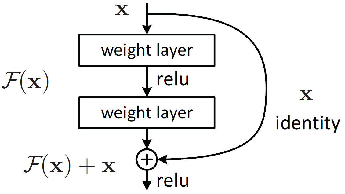
This simply consists of forwarding the activation of a certain layer to a deeper layer in the network; as we can see in Fig. 1, the result of the activation coming from a previous layer is added to that of a deeper one. This simple expedient avoids problems with the numerical gradient in the optimization phase, and prevents the loss of information during the training of very deep networks. We will see later that, although this method makes it possible to reuse some prior knowledge without having to start from scratch each time with the training of a convolutional network, transfer learning is not always an efficient procedure for solving an image classification task.

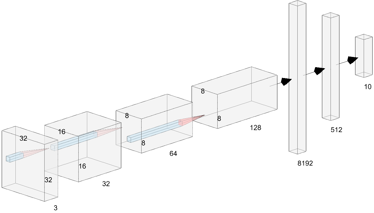
Second approach: custom convolutional network. As a second method, we will use a convolutional network created specifically for the task, and trained on the dataset from scratch. Its layers are defined as follows:

• INPUT
• CONVOLUTIONAL 1
  • Number of filters: \(32\)
  • Kernel size: \( 3\times3 \)
  • Padding: SAME
  • Stride: 1px
• RELU
• MAX POOLING 2D
• CONVOLUTIONAL 2
  • Number of filters: \(64\)
  • Kernel size: \( 3\times3 \)
  • Padding: SAME
  • Stride: 1px
• RELU
• MAX POOLING 2D
• CONVOLUTIONAL 3
  • Number of filters: \(128\)
  • Kernel size: \( 3\times3 \)
  • Padding: SAME
  • Stride: 1px
• RELU
• FULLY CONNECTED 1
  • Input nodes: \( 8192 \;(8\times8\times128) \)
  • Output nodes: \(512\)
• BATCH NORMALIZATION
• RELU
• DROPOUT (\(p=0.5\))
• FULLY CONNECTED 2
  • Input nodes: \(512\)
  • Output nodes: \( 10 \)
• DROPOUT (\(p=0.5\))

The loss function used for all the trainings is the Cross Entropy Loss, also called Log Loss which, in the generic multi-class case with \(n\) classes, is formulated as follows: $$L=-\frac{1}{n}\sum_{i=1}^ny_{i}\log(p_{i})$$ where \(p_i\) denotes the softmax probability for class \(i\), and \(y_i\) is the truth label. It is by no means the only loss function available; there are others such as the hinge loss, the logistic loss and more, but this one is certainly among the most widely used; as stated in Pattern Recognition and Machine Learning¹¹, using the cross-entropy error function instead of the sum-of-squares for a classification problem leads to faster training as well as improved generalization. After the first two convolutional layers, we used MAX POOLING to reduce the resolution of the filters and make the network invariant to translations of the input, taking only the maximum of the values of the region it belongs to. This also increases the receptive field of the deeper neurons, allowing the network to handle more semantic information at a time in the subsequent filters, creating feature maps that are progressively more complex.

DROPOUT layers were inserted after both of the last two fully connected layers, just after the nonlinearity; this was the original approach of the authors who proposed this type of layer¹². More recent research shows the advantages obtainable by using this type of layer even after the first convolutions, always after the nonlinearities, although with much lower values of \(p\), around \(0.1-0.2\)¹³. The purpose of this type of layer is to regularize the network, forcing it to adapt to connections that are randomly broken with probability \(p\) at each forward step (and only during training). The consequence is that at each training step, the layer the dropout is applied to is seen and treated as having a different number of nodes and a different configuration than at the previous step. The end result is to approximate or, better, simulate the training of multiple networks with different architectures, in parallel.
In addition, a BATCH NORMALIZATION layer was inserted after the first fully connected layer to help the convergence and stability of the network, through re-centering and re-scaling of its inputs¹⁴. It was believed that this practice reduced the internal covariate shift of the parameters, a problem related to network initialization, but more recent studies show that the reason for the increase in performance is not due to this normalization effect¹⁵. In a recent publication, it is shown that by using a gradient clipping technique and through some tricks in the tuning of certain hyperparameters, the need for batch normalization becomes marginal¹⁶.

Experiments

Four different trainings were performed:

• 1-2) ResNet-18:

  • Optimizer: Adam and SGD; best model chosen.
  • Learning rate scheduled from \(1 × 10^{-3}\) to \(8 × 10^{-5}\)
  • Loss: Cross Entropy

• 3) Custom net 1:

  • Optimizer: Adam
  • Learning rate fixed at \(1 × 10^{-3}\)
  • Loss: Cross Entropy

• 4) Custom net 2:

  • Optimizer: Adam
  • Learning rate scheduled from \(1 × 10^{-3}\) to \(8 × 10^{-5}\)
  • Loss: Cross Entropy

All nets were trained for a total of 30 epochs, for a twofold reason: on one hand, the training time started to become almost prohibitive for a larger number of epochs; on the other hand, it was observed that increasing the epochs (and decreasing the learning rate, in the runs with a scheduler) brought no further benefit to the test accuracy metric. An early stopping technique could also have been implemented, but it was deemed useful to let the training complete all of the 30 scheduled epochs anyway, both to verify that nothing anomalous was happening and because better results could still have emerged thanks to the continuous decrease of the learning rate.

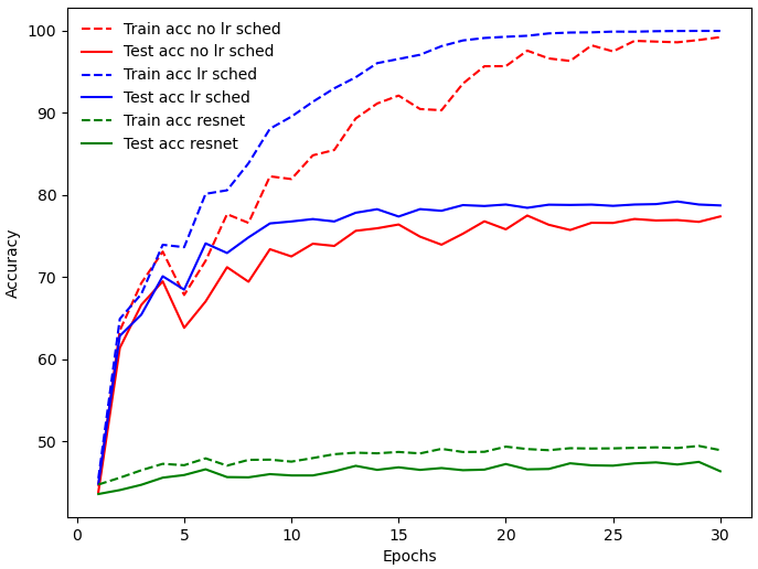
Custom network results. Let us then analyze the results in this graph: as we can see, after about 10-15 epochs the test accuracy has already reached its final value, both for the classifier with the learning rate scheduler and for the one without, and it sits around 79% for the network with the scheduler versus 77% for the network without it. The difference is small, but it remains detectable throughout all the training epochs, thus demonstrating the usefulness of optimizing with a progressively decreasing learning rate. Another thing to take into account is that the accuracy on the training set goes up to 99% in both cases, meaning the models completely overfit the training data.

Transfer learning results with ResNet-18. As for the results obtained with the second architecture — the one that uses ResNet-18 as a feature extractor — they unfortunately leave much to be desired. Although a decreasing learning rate was used in this case as well, the accuracy almost immediately reaches its maximum: the accuracy on the test set is close to 48% at most, and the one on the train set settles around a more stable 50%. Trying to investigate the problem, I noticed that the network was pre-trained on the ImageNet dataset^{10 17}, which consists of millions of images, divided into more than 20000 categories. The theory I have thus formulated is that the relatively shallow depth of the network may have caused a bottleneck in the representational power of the network itself with respect to such a large amount of information, but it is only a hypothesis.
Let us now look at the confusion matrices: for the custom architecture we will consider only the model that makes use of the progressive learning rate, as it reports better results overall.

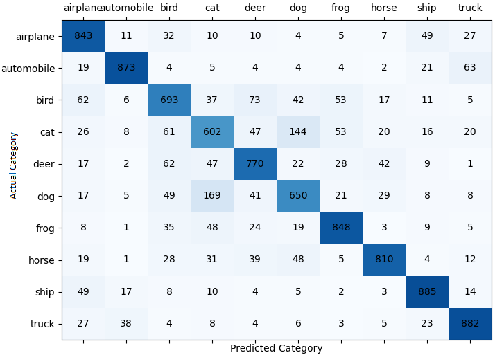
As we see from Fig. 3, the classes are identified with more than acceptable confidence; given their low resolution, it is interesting but predictable to see that the classes most easily confused with each other are “cat” with “dog”, “airplane” with “bird” and “ship” (probably because of the often mostly-blue background), and “automobile” with “truck”, likely due to some common visual features, such as wheels or doors.

As the example shown in Fig. 4 demonstrates, not all images are significantly different from each other from a visual point of view; some of them can easily be classified incorrectly even by humans¹⁸. This explains the false positives outside the diagonal of this matrix.

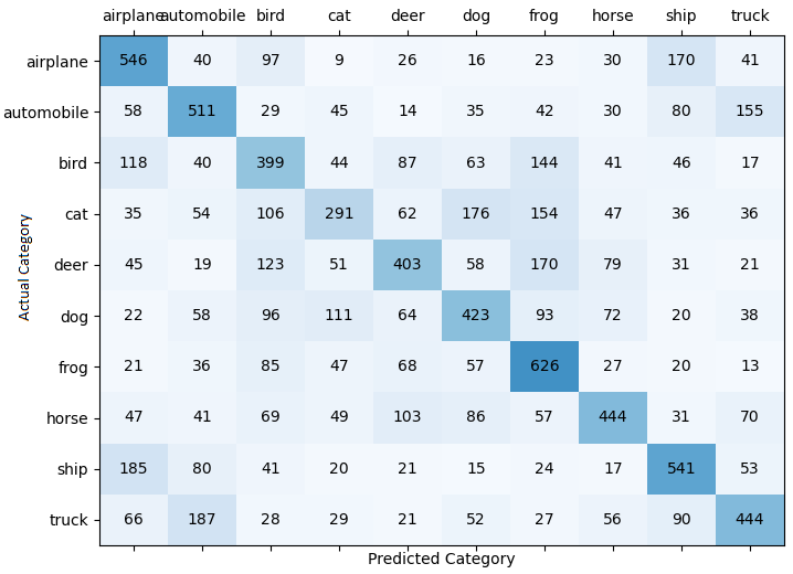
In the latter case, as we expected given the Top-1 accuracy results in Fig. 2, the classifier struggles much more to correctly identify the classes the various images belong to. One notices the same confusions discussed above, but much more pronounced, and outliers can also be seen: while we might well expect some low-resolution “cat” images to be mistaken for images of “dog”, we certainly do not expect these “cat” images to be identified as “frog” with a frequency that is half that of the correct classifications.

On computational complexity. I think it is important to mention the issue of computational resources: the custom convolutional network seen in this project was definitely not on par with the depth and performance of the convolutional networks at the top of competitions such as the ILSVRC¹⁹. As we can see from Fig. 5²⁰, more layers — and thus more parameters — does not automatically mean better performance, as it could just mean more problems during optimization. In any case, as the depth of the network increases, a greater representational capacity can undoubtedly be achieved; something I was not able to experience since even just adding one additional convolutional layer (thus bringing the total to four) already manifested the physical limitations of the computer in my possession, despite it having a graphics card with 2GB of dedicated video memory. With the configuration just seen, memory usage is around 1.3-1.5 GB during the training phase, with a batch size of 64 images. By reducing this hyperparameter you can reduce memory usage although, against my expectations, only rather marginally.

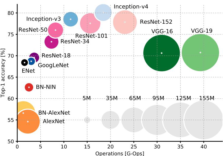
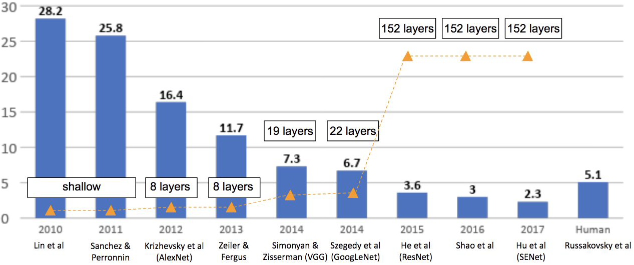
Also related to the ILSVRC, we can see from Fig. 6²¹ how with ResNet there has been a “depth revolution” of convolutional networks: the number of layers exploded, and the classification performance doubled. The real revolution, however, is that all this did not also bring an explosion of the parameters — and thus of the size and complexity of the networks; as we can see from Fig. 5, the number of parameters and the operations required for the forward pass remained quite contained, or even decreased in some cases.

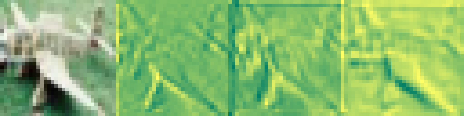
Finally, let us visually explore some of the feature maps extracted from the dataset. Also called “activation maps”, these indicate the activation response of a given filter to the passage of an image through the convolutional network. In Fig. 7 we can see the responses of feature map number 6 in the various layers, and how the edges of the plane’s wings are made more and more pronounced.

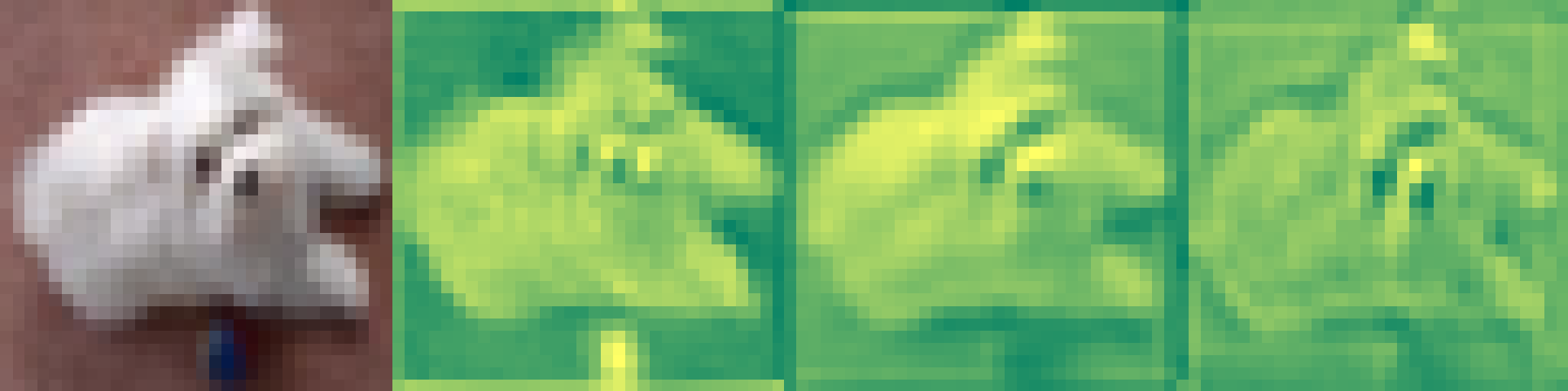
In Fig. 8, we can see how the 11th feature map succeeds in removing some of the background elements, as they are not informative for the identification of the dog class, while maintaining a high response on the contours of the dog’s body and on the muzzle.

Conclusion

From the results we can therefore conclude that even a network with a shallow architecture, such as the custom one discussed, can achieve a more than satisfactory accuracy despite its simple nature. On the other hand, the increase in complexity and in the required computational resources quickly proved to be an obstacle to experimentation, preventing me from going beyond just 3 convolutional layers.
As for the network obtained from the pre-trained ResNet, the performance is unfortunately disappointing. As discussed earlier, the weights of all the layers of this network except the last, fully connected one are derived from a training on a dataset different from the one used for the rest of the experiment, namely ImageNet¹⁰. Only the last dense layer was retrained to fit the task; this approach, however, did not prove productive. Nevertheless, this absolutely does not mean that the transfer learning technique is not useful; rather, it means that it should be used with more care, for example with a fine tuning of the parameters instead of keeping them frozen — in other words, starting from a minimum and, instead of remaining there, moving toward a better minimum through multiple optimization steps.
Finally, it is worth mentioning that the classes that give the network the most difficulty are, of course, the visually closest ones, such as cat and dog, or car and truck; and, as a matter of common background, even airplane is confused a significant number of times with images of the bird and ship classes; an example is the one shown in Fig. 4.
Incremental work on these results would be conceptually very easy to realize, and could include increasing the number of convolutional layers, removing one of the fully connected layers, and a better fine tuning of the parameters in the case of transfer learning. In practice, this would require additional hardware resources, given what was discussed above.